The HaCI algorithm, or Harmonic Contour Integration, provides a compact method for extracting edges from RGB images by mimicking biological vision processes. Developed by RenderBear, the algorithm processes images through a distributed pipeline that moves from pixel-level contrast to high-resolution ridge back-projection. It offers a specialized alternative to standard edge detection, balancing biological plausibility with measurable performance on benchmarks like BRIND and BIPED.

This image serves as a representative example of the RGB input data that the HaCI algorithm processes through its four-stage pipeline.
The Four-Stage Pipeline
The algorithm begins at the L0 stage, where each pixel is compared to its eight neighbors using a learned luminance/chroma metric. This contrast is divided by a local spatial pool of contrast, creating a per-pixel harmonic field. In the L1 stage, these harmonics are summed over overlapping patches on a sparse cell grid to produce orientation-tuned responses.
The 'Seed' stage applies biological principles like Naka–Rushton gain control and association fields. This step scales responses based on neighboring cells along a contour and uses flank suppression to divide out parallel contours. This process ensures that lone edges are preserved while textures and gratings are dampened. Finally, the 'Render' stage splats these cell responses back to full resolution using learned 1D kernels to produce a soft boundary map.
“A compact, fully distributed algorithm that extracts edges from RGB images through four stages:”
— GitHub - RenderBear/haci: A compact, fully distributed algorithm that extracts edges from RGB images
Benchmark Performance
HaCI was evaluated on the BRIND test set, which consists of 200 images re-annotated for different discontinuity types. The algorithm's NMS-thinned map achieved an ODS (Optimal Detection Score) of 0.7179 and a precision of 0.6791. The raw soft map produced by the renderer showed a slightly lower ODS of 0.7158.

This figure illustrates the final output of the HaCI pipeline, showing the extracted edges and contours.
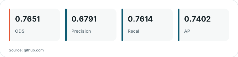
Chart drawn by HN Digest from figures reported by github.com; values are shown as written in the source.
The project also supports testing on the BIPED and NYUDv2 datasets. For the NYUDv2 dataset, the evaluation uses a matching distance of 0.011, reflecting the less precise localization of its ground truth compared to the stricter 0.0075 tolerance used for the BRIND and BSDS500 benchmarks.
Hardware Efficiency and Trade-offs
The algorithm demonstrates efficient execution on modern hardware, specifically Apple's Metal Performance Shaders (MPS). For a 1920x1080 resolution, the system requires 233 MB of host memory and 2.2 GB of GPU memory, completing inference in 459 ms. The renderer's splat and gradient operations are implemented as Metal kernels to ensure consistency with CPU paths.
A primary trade-off exists between the raw soft map and the NMS-thinned map. While the thinned map improves precision and recall by removing noise, the raw map provides a continuous boundary representation. The source does not provide a direct head-to-head comparison with state-of-the-art non-bio-inspired deep learning models, focusing instead on the internal consistency of the HaCI pipeline.