When PyTorch builds a computation graph for a machine learning model, it must decide which operations to store in memory and which to recompute to stay within a specific RAM budget. This is framed as a 0/1 knapsack problem: each operation is an 'item' with a memory cost and a runtime 'value.' The goal is to select a set of operations to save that maximizes total time savings without exceeding the available memory capacity. While PyTorch traditionally uses a dynamic programming (DP) approach called `dp_knapsack` to solve this, the standard implementation requires allocating a full 2D table of shape (number of items, max weight), which can lead to memory exhaustion on large models.

This image illustrates the knapsack problem mentioned in the first paragraph, where operations are treated as items with memory costs and runtime values.
To address this, Jędrzej Maczan introduced `dp_knapsack_sliding_hirschberg`, a solver that significantly reduces the memory footprint of the planning phase itself. The implementation utilizes two primary optimizations. First, it employs a 'sliding window' trick, which reduces the space complexity of the DP table by only keeping the current and previous rows in memory. Second, it incorporates the Hirschberg algorithm, a divide-and-conquer approach that eliminates the need for a costly backtracking step. Instead of building a massive table and tracing back to find the optimal items, the Hirschberg method recursively splits the problem into smaller sub-problems, identifying the optimal split points until the final set of saved operations is determined.
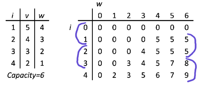
This figure explains the first optimization mentioned in the second paragraph: using a sliding window to minimize the memory footprint of the DP table.
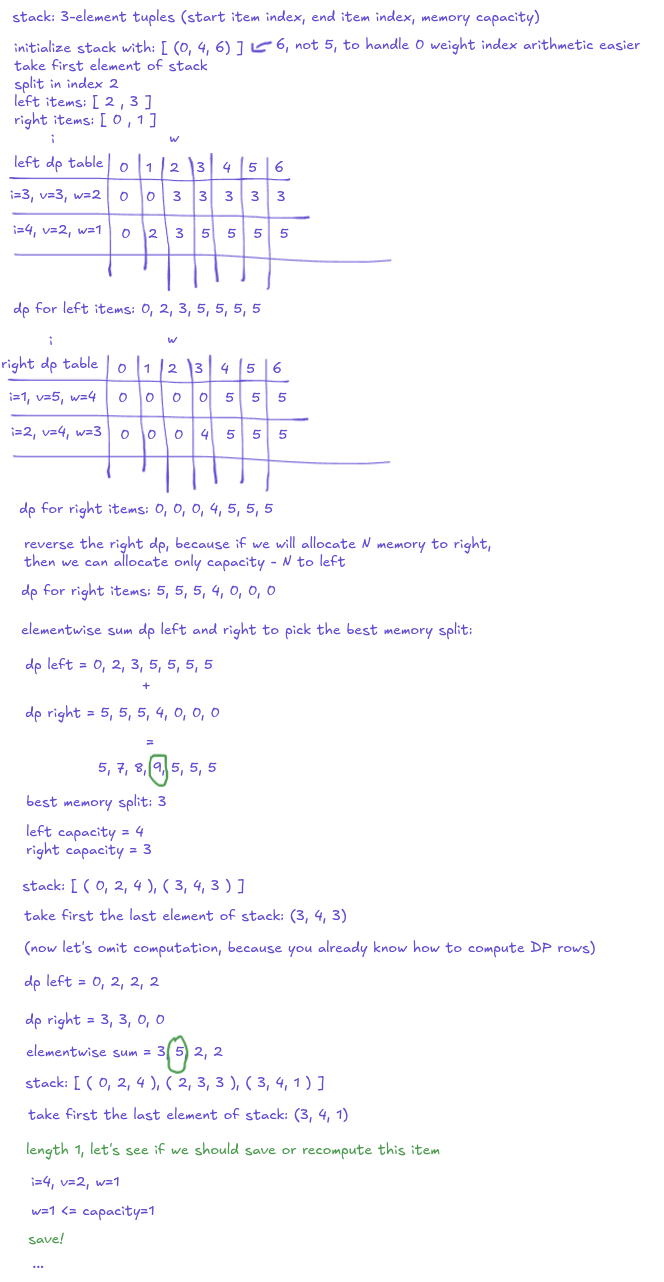
This visual supports the second optimization described in the second paragraph, showing how the Hirschberg method recursively splits the problem.
In practical testing, this change allows the solver to handle problems with 2,000 items on a machine with 64GB of RAM—a task where the original `dp_knapsack` solver would crash with only 100 items. While the new solver provides an exact solution and roughly a 37% speedup over the baseline, it is not the fastest available method. For users who can include external dependencies, the Integer Linear Programming (ILP) solver via SciPy is significantly faster. However, for those restricted to standard PyTorch distributions, `dp_knapsack_sliding_hirschberg` offers a robust way to manage memory-intensive models without the overhead of the traditional DP table.
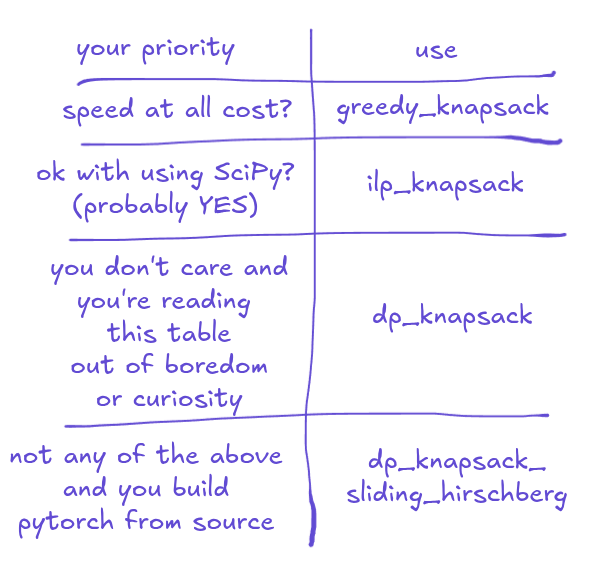
This image illustrates the practical testing results and the comparison between the new solver, the baseline, and external ILP solvers discussed in the final paragraph.